Geoid modeling calculations
Research question: What is the NOAA procedure for generating a geoid model?
NOAA’s NGS geoid team receives all the available gravity datasets (space, airborne, land, and marine) collected over North America and the Pacific Ocean. The datasets have been cleaned for outliers and errors related to the platform or the instrument and are reduced based on the error characteristics of each data set. The U.S. federal agencies collaborate on different geodetic efforts as a geodetic Community of Practice. For example, NOAA shares its airborne gravity data with other federal agencies within the U.S., and similarly the National Geospatial-Intelligence Agency (NGA) and the National Aeronautics and Space Administration (NASA) share their marine gravity and space gravity missions data acquired, respectively.
For the development of a seamless geopotential surface over North America, NGS geoid team works closely with counterpart offices in Canada and Mexico on geoid model development and sharing data. The outcome of the international collaboration is to produce a high quality geoid that has a seamless geopotential surface from the Atlantic Ocean to the Pacific Ocean, providing coverage over all of the U.S. and its territories. The geoid products are used in many NOAA operational applications, such as initializing coastal and ocean modeling (flooding, inundation, surge, and tides), planning and predicting satellite orbits, and also for defining a seamless reference system over water and land.
A key principle in the NOAA geoid modeling is the use of the Stokes Integral for transforming gravity anomalies into a vertical reference system that can link the location of the geopotential surface to a reference ellipsoid. Stokes’ Integral is part of Stokes' Theorem, which is one of a family of mathematical results that link a property of a volume to a property on its boundary. For example, we can quantify the amount of water in a vessel by the volume of water. This volume changes by exactly the amount that is added or removed. In gravity, Stokes' theorem takes this idea and generalizes it. The Stokes’ integral requires gravity values across the entire planet’s surface as an input. Over land, millions of terrestrial gravity observations provide input for the geoid model. Over oceans, the main data sources for gravity anomalies are inferred from satellite altimetry measurements of the shape of the ocean. These surface data points come from a variety of sources, so models of gravity derived from airborne platforms (GRAV-D) and dedicated satellite gravity missions (GRACE, GRACE-FO, GOCE) are used to harmonize them across hundreds to thousands of kilometers. Finally, digital elevation models are used to fill in the gaps in the terrestrial gravity data and control for the fine-scale contributions of surface topography to the gravity field.
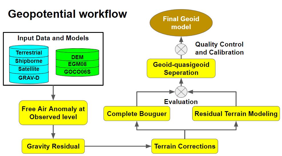
The NGS geoid modeling workflow is driven by removing as much of what we know about the global geopotential field from the gravity data and transforming the remaining signal into corrections to the geoid. In general, there are five key steps in the NGS geoid modeling workflow for transforming gravity measurements into geoid undulations:
-
Compute Free-Air Anomalies from observed gravity
In order to process different sources of gravity data over the same reference, the gravity values (acceleration) are corrected for their geographic location and elevation on the Earth’s surface with respect to a known mathematical vertical reference system, an ellipsoid. The variation of the gravity values are first corrected based on the geographic location of the observation with respect to the equator using a reference ellipsoid (i.e., GRS-80). This step, known as the normal gravity correction or latitude correction, accounts for the observation’s location related to the non-spherical shape of the Earth and because the angular velocity of a point on Earth’s surface decreases from a maximum at the equator to a zero at the poles.
Next, the gravity observations are corrected for the normal gravity that is a function of latitude and altitude of the observation. This process known as the Free air correction accounts solely for variation of the location of observation from the center of the Earth (i.e., the distance from the center of the Earth), but does not take into account the density difference of rock present between the observation point and reference ellipsoid. A positive free-air correction is subtracted from locations above the reference ellipsoid. The product of this correction is the Free-Air anomaly at the observation level, which provides the difference between the observed gravity values and the gravity acceleration predicted by an ellipsoidal gravity model.
-
Subtract a Reference Model to obtain Gravity Anomaly Residuals
NOAA’s geoid model only covers part of the Earth’s surface. This becomes a challenge for using Stokes’ Integral, which requires gravity values available for the entire planet’s surface. It is possible to bypass this requirement by subtracting a known global gravity model, thereby setting all the gravity outside of the area of interest to a zero value. The NOAA geoid team calculates a reference global geopotential model (i.e., a reference model) in order to calculate the gravity anomaly residual, i.e., the difference between the calculated Free-Air anomalies to the reference model. By looking at the difference between the observed values and the reference model, it is possible to exclude observations outside of the area of interest, such as satellite gravity observations.
NGS develops its reference model by blending existing global geoid models with the most recent satellite models and GRAV-D airborne data. These models are defined using spherical harmonics. Spherical harmonics mathematical functions allow NGS to simulate a reference model anywhere above Earth’s surface in order to account for most of the observed gravity signal. It is possible to simulate multiple reference models using different configurations and selecting the best fitting reference model for subtracting its values from the Free-Air anomaly. The end product from this step is a gravity anomaly residual layer. NGS uses the GRAV-D airborne gravity data to enhance the global geopotential model that contains information from satellite and terrestrial gravity.
-
Subtract Topographic Effects using Digital Elevation Models
The Free-Air anomaly correction and the use of a reference model are able to account for coarse-resolution features (>10 km). However, high-resolution spatial variations caused from vertical changes of the topography are still present in the gravity field. These spatial variations are on the order of 10s to 100s of meters. It is possible to remove these contributions from the gravity data by using high-resolution (10s of meters) digital elevation models produced from common photogrammetry and remote sensing technologies (e.g., airborne lidar, space Interferometric Synthetic Aperture Radar (InSAR), and traditional aerial photogrammetric techniques). Subtracting the topographic signal leaves a smooth, easy-to-interpolate gravity field, which largely reflects subsurface variation in crustal density and thickness. The topographic-effect-corrected gravity anomalies are also used for gravity data interpolation and fill in gravity signals where gravity data are missing.
The NOAA geoid team applies, in parallel, two different approaches for topographic effect to the Residual Gravity datasets. Each of the topographic correction approaches has advantages and limitations. By using a parallel approach, the NOAA geoid team is able to evaluate how well the correction performed and if one approach provides a better result. The two approaches used in NOAA include:
- Complete Bouguer approach subtracts the gravitational attraction of the rock between the observation location and the geoid over land observations. For marine gravity observations, the Bouguer correction accounts for the difference in density of water and a specified rock density. The Bouguer corrections also account for isostasy, where higher terrain requires a thicker crust in order to compensate for buoyancy over the mantle.
- The residual terrain modeling (RTM) technique (Forsberg, 1981), which removes the reference (mean) topography and works on the residual terrain exclusively. This method has been widely applied in the gravity field determination.

Schematic illustration for Tidal, Free Air, and Topographic corrections on survey gravity datasets -
Transform Residual Gravity Anomalies into Surface Geopotential using the Stokes Integral
For developing a model that can produce geopotential surfaces, the terrain-corrected residual gravity data need to be transformed from acceleration into geopotential units of measure, the NOAA geoid team applies the Stokes’ Integral, which is an implementation of Stokes’ Theorem. The Stokes’ integral transforms a field of observed gravity anomalies (in m/s^2) at Earth’s surface into a field of predicted geopotential anomalies (in m^2/s^2) that may be evaluated anywhere above the surface.
It is important to note that the outcome from the Stokes’ Integral in the NGS process are transformed gravity anomalies that only give residual geopotential anomalies, i.e., corrections to the known differences in the geopotential field. To recover the full geopotential field that defines the geoid, these residual anomalies must be added to the geopotential anomalies computed from the reference model and the topography model subtracted in the previous steps. These modeled geopotential fields are added back to the residual anomalies to obtain the full, corrected, geopotential. The final output of this step is a grid of geopotential anomalies evaluated at the topographic surface.
-
Compute the Geoid from Surface Geopotential Using the Geoid-Quasigeoid Separation
Because NOAA conducts its gravity processing using the contemporary geoid theory, all the corrections and calculations are done at the Earth’s surface. This minimizes assumptions about subsurface density to the greatest extent possible. Dividing the disturbing potential at the surface by the full-field acceleration of normal gravity at the surface gives a height reference surface called the “quasigeoid.” Unlike the geoid, the quasigeoid is not an equipotential surface. To transfer geopotential values at the surface to the ellipsoid and obtain an equipotential surface, we must account for the topographic mass between the surface and the geoid. Therefore, the digital elevation model and gravity data are used to compute the geoid-quasigeoid separation term, which is added to the quasigeoid to obtain the geoid.


Quality Control and Calibration
The final geoid model is checked against available independent validation data sets, including survey marks where heights have been measured with both GNSS and leveling. NGS’s Geoid Slope Validation Surveys, which use GPS, spirit leveling, gravity, and astronomical deflections of the vertical to assemble empirical geoid profiles are the ultimate standard of geoid accuracy. The final geoid product is used as a starting point for computing the deflection of the vertical, which indicates the direction of gravity at the surface with respect to the ellipsoid normal. Deflections of the vertical may be used for inertial navigation and transforming local survey data into a global reference frame.
Finally, the geoid must be calibrated to best fit mean sea level at its 2020.0 reference epoch. Its long-term, time-dependent changes due to the changing distribution of mass near Earth’s surface are determined by satellite gravity missions and in-situ measurements (Geoid Monitoring Service).
Peer Review Publications and Conference Presentations
Ahlgren, K., D. van Westrum, and B. Shaw. 2024. “Moving mountains: reevaluating the elevations of Colorado mountain summits using modern geodetic techniques,” J Geod 98, 29.https://doi.org/10.1007/s00190-024-01831-8
Groten, E. 1981., Precise Determination of the Disturbing Potential Using Alternative Boundary Values NOAA Technical Report NOS 90 NGS 20 Rockville, Md. August 1981
Forsberg, R. and C. Tscherning. 1981., “The use of height data in gravity field approximation by collocation,” J Geophys Res 86(B9):7843–7854
Li, X. 2021. “Leveling airborne and surface gravity surveys,” Appl Geomat 13, 945–951. https://doi.org/10.1007/s12518-021-00402-2
Li, X., J. Huang, R. Klees, R. Forsberg, M. Willberg, D.C. Slobbe, C. Hwang, and R. Pail. 2022. “Characterization and stabilization of the downward continuation problem for airborne gravity data,” J Geod 96. https://doi.org/10.1007/s00190-022-01607-y
Li, X. et al. 2022. “Using High–Low Flight Gravity Data to Improve Geoid Model Precision: A Case Study in U.S. Virgin Islands (July 2021),” in IEEE Geoscience and Remote Sensing Letters, vol. 19, pp. 1-3, 2022, Art no. 8023203, https://doi.org/10.1109/LGRS.2021.3129374
Lin, M., and X. Li. 2022. “Impacts of Using the Rigorous Topographic Gravity Modeling Method and Lateral Density Variation Model on Topographic Reductions and Geoid Modeling: A Case Study in Colorado, USA,” Surv Geophys 43, 1497–1538. https://doi.org/10.1007/s10712-022-09708-1
Saleh, J., X. Li, Y.M. Wang, D.R. Roman, and D.A. Smith. 2013. “Error analysis of the NGS’ surface gravity database,” J Geod 87, 203–221. https://doi.org/10.1007/s00190-012-0589-9
van Westrum, D., K. Ahlgren, C. Hirt, S. Guillaume. 2021. “A Geoid Slope Validation Survey (2017) in the rugged terrain of Colorado, USA,” J Geod 95, 9. https://doi.org/10.1007/s00190-020-01463-8
Wang, Y.M., M. Veronneau, J. Huang, K. Ahlgren, J. Krcmaric, X. Li, and D. Avalos-Naranjo. 2023. “Accurate computation of geoid-quasigeoid separation in mountainous region – A case study in Colorado with full extension to the experimental geoid region.” Journal of Geodetic Science 13, 1. https://doi.org/10.1515/jogs-2022-0128, https://repository.library.noaa.gov/view/noaa/54994
Wang, Y.M., M. Veronneau, J. Huang, K. Ahlgren, J. Krcmaric, X. Li and D. Avalos-Naranjo. 2022. NOAA Technical Report NOS NGS 78 National Oceanic and Atmospheric Administration National Geodetic Survey Technical Details of the Experimental GEOID 2020, https://geodesy.noaa.gov/library/pdfs/NOAA_TR_NOS_NGS_0078.pdf
Wang, Y.M., L. Sánchez, J. Ågren, et al. 2021. “Colorado geoid computation experiment: overview and summary,” J Geod 95, 127. https://doi.org/10.1007/s00190-021-01567-9
Wang, Y.M., J. Saleh, X. Li, and D.R. Roman. 2012. “The US Gravimetric Geoid of 2009 (USGG2009): model development and evaluation,” J Geod 86, 165–180. https://doi.org/10.1007/s00190-011-0506-7
Wang, Y.M., X. Li, K. Ahlgren, and J. Krcmaric. 2020. “Colorado geoid modeling at the US National Geodetic Survey,” J Geod 94, 106, https://doi.org/10.1007/s00190-020-01429-w
Wang, Y.M., M. Veronneau, J. Huang, K. Ahlgren, J. Krcmaric, X. Li, and D. Avalos-Naranjo. 2023. “Accurate computation of geoid-quasigeoid separation in mountainous region – A case study in Colorado with full extension to the experimental geoid region,” Journal of Geodetic Science. 13. https://doi.org/10.1515/jogs-2022-0128
Yang, M., X. Li, M. Lin, X-L Deng, W. Wei Feng, M. Min Zhong, C.K. Shum, and D.R. Roman. 2023. “On the harmonic correction in the gravity field determination,” J Geod 97, 106. https://doi.org/10.1007/s00190-023-01794-2
